Leetcode Problem: Map of Highest Peak

Problem Description

You are given a matrix isWater of size m x n where:

• isWater[i][j] == 0: This cell represents land.
• isWater[i][j] == 1: This cell represents water.

The input specifies where water and land cells are located, but it does not specify the heights of the land cells. Your task is to assign heights to the land cells following these rules:

1. Water cells must have a height of 0.
2. Any two adjacent cells (north, south, east, west) must differ in height by at most 1. This ensures a smooth gradient of heights between neighboring cells.
3. Assign heights to land cells in a way that maximizes the highest height in the matrix.

Your goal is to return a matrix height of size m x n where height[i][j] represents the height of cell (i, j) while following the rules.

---

Examples

Example 1:

Input:
isWater = [[0,1], [0,0]]
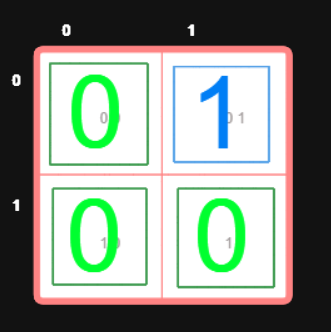Output:
height = [[1,0], [2,1]]
Explanation:

• The water cell at (0,1) has height 0 (rule #1).
• Its adjacent land cells (0,0) and (1,1) have heights 1 and 1, differing by exactly 1 (rule #2).
• The bottom-left cell (1,0) has height 2, which is the highest possible height while meeting the adjacency rule (rule #3).

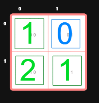
Example 2:

Input:
isWater = [[0,0,1], [1,0,0], [0,0,0]]

Output:

height = [[1,1,0], [0,1,1], [1,2,2]]

Explanation:

• All water cells (0,2) and (1,0) have height 0.
• Land cells around the water are assigned increasing heights, forming a gradient that satisfies the adjacency rule.
• The highest height in this matrix is 2.

---

Approach to Solve the Problem

1.Initialization:
Start by creating the height matrix where all cells are initially unassigned. Assign 0 to all water cells since water must have height 0.

2. Use BFS (Breadth-First Search):
   Perform a multi-source BFS starting from all water cells (height = 0) simultaneously.
   • Push all water cells into a queue.
   • As you process each cell, assign heights to neighboring land cells if they are not already assigned.
   • Ensure the height of a neighboring cell is exactly 1 more than the current cell’s height.
3. Propagation of Heights:
   The BFS will propagate heights outward from water cells.
   • Cells farther from water will have higher heights.
   • This ensures that the maximum height is reached at the farthest land cells.
4. Output the Matrix:
   Once BFS completes, the height matrix will be filled, and the maximum height will naturally be achieved.

---

Key Observations

1. Water cells act as the starting point (height 0) for spreading heights to the surrounding land.
2. The farther a land cell is from water, the greater its height, due to the adjacency constraint.
3. Using BFS ensures that each cell is processed in the shortest possible path from the water, which guarantees that heights are maximized correctly.

---

Constraints

• Matrix size: 1 <= m, n <= 1000.
  This ensures the algorithm must be efficient to handle large matrices.
• At least one water cell exists (isWater contains at least one 1).

---

Why BFS?

• BFS is ideal for problems requiring shortest-path propagation, like this one, where heights depend on the shortest distance from water.
• It processes all cells layer by layer, ensuring heights increase uniformly from water.

---

Complexity

1. Time Complexity:
   • BFS processes each cell exactly once, so the time complexity is O(m * n).
2. Space Complexity:
   • The queue used in BFS requires space proportional to the number of cells, which is also O(m * n).

This ensures the solution is efficient and scalable for large inputs.

— Written by Saurabh Patil • B.Tech CSE • Software Developer